-Neil Peart
Modern day warrior with a mean, mean stride
TL;DR
Machine learning has lots of models touted for their predictive power, despite having the straightforward interpretability of a Jackson Pollock piece. Here I explore LIME, a model-agnostic method for interpreting predictions.
LIME
(Local Interpretable Model-Agnostic Explanations)
The Tale of LIME
When the world was young, there was linear regression. And all the statisticians in the land were happy making unreasonable assumptions and getting clear linear effects of features on target variables (or "x" and "y" in the language of the ancients). Then came a dark cult called the "computer scientists" who used their dark magic to perform millions of calculations per second, enabling complex numerical estimations. But this dark magic was cursed -- you could only know what the prediction was, not the reason behind it!
Then, in 2015, a powerful trio of wizards named Ribiero, Sing, and Guestrin came up with a spell to combat the dark ether surrounding the computer scientists' predictions. And thus LIME was born.

Actually explained
The rise of extreme reduced-form models has led to a frenzy of prediction. XG-boost and neural nets are two of the current all-stars in the field, but trying to interpret these models has been a sticking point. And with the toolbox of data-scientists ever-growing, it's important not to forget the importance of understanding the driving factors behind predictions.
XGBoost and Random Forests
The main method for XGBoost, and other random forests, is calculating feature importances. Though methods vary, it's often based on a methodology from Brieman and Friedman.[1] The idea is that you track all of the paths through the trees, calculating the reduction in error attributable to that split weighted by the number of observations flowing through the split. A thorough description (as well as a great many other thorough descriptions) can be found in The Elements of Statistical Learning[2]. (i.e. the ML bible)
This is handy, but doesn't give you much an idea of it's relationship to the individual predictions themselves.
Neural Nets
Neural nets have their own set of problems with interpretability. Neural nets are also basically a big plate of "feature-weight and linear/non-linear mix" spaghetti. There are a number of ways that people attempt to visualize this. With nets for images, for example, there is an ability to see what patterns certain filters are picking up. But again, it doesn't do much for the end result.
Others
There are a number of other models that can be difficult to interpret (SVMs for example). The model-agnostic nature of LIME makes it a powerful tool no matter what kind of problem you're working on.
LIME
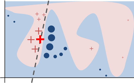
So how does LIME work? Firstly, as the name implies, it's focused on local interpretation, i.e. a single observation. The idea is that if you can perturb the features of that observation, you can fit a simpler, interpretable model around it. For instance, a simple linear model where your coefficients are simply the marginal effects of individual feature perturbations! I defer to the wonderfully titled Why Should I Trust You? for the details.

Ok, so what?
That's an excellent question, Tyler! (thanks, Tyler!) The answer has a few parts to it:
- Many models don't mean much without interpretability.
- Imagine you're trying to predict whether a customer will ever return to buy something again. Although the probability itself may be useful, it's not a super actionable number. What is making it more or less likely they'll come back? How strong is the effect for this person vs others?
- There's the question begged by Ribiero, et. al., "Why should I trust you?".
- Although these models can be very powerful, they can also latch onto noise or be thrown off by spurious correlations. At the end of the day we all live in the real world and problems should (almost always) have to pass a common sense smell test.
- There are other factors that may not be in the model but that may mean something to a researcher for future modeling.
- There could be structural changes in the way processes behave and with a black-box you can't predict when it might happen until your model accuracy goes down the tubes.
- Let's say you're modeling horse races. Your model works great except every few years or so for a full season. It turns out that the most important features are actually highly dependent on the weather and you're getting thrown off by el nino! For example, rain isn't a big deal for a horse as long as it doesn't have to run in it every single day. Or during particularly rainy seasons the soil softens over time, so even sunny days are hard to run in.
There are a host of reasons, but in general it's just helpful to know what's going on when you're modeling. And the appealing thing about lime is that it's model agnostic, so you can utilize it almost wherever you need!
LIME in action!

A quick heads up: due to the length of the python scripts in this, I'm to put a link to them here and then simply describe the results. Though I do encourage all of my (I assume) millions of fans to try it yourself!
Example 1: Tell me what I already know
(Linear Regression)
Reproduction of the OLS
"...but linear regression is easily explainable already?"
Exactly. Which makes it the perfect pedagogical tool for LIME.
For this example I'm using the classic Boston Housing Dataset. A simple regression should get us what we need:
Response Var:
  medv     Median value of owner-occupied homes in $1000's

Features:
  nox      nitric oxides concentration (parts per 10 million)
  rm       average number of rooms per dwelling
  dis      weighted distances to five Boston employment centres
  ptratio  pupil-teacher ratio by town
  b        1000(Bk - 0.63)^2 where Bk is the proportion of blacks by town
  lstat    % lower status of the population


Model:
  medv ~ nox + rm + dis + ptratio + b + lstat + constant

                            OLS Regression Results
==============================================================================
No. Observations:                 506        Df Residuals:                 499
R-squared:                       0.715       Df Model:                       6
==============================================================================
                 coef    std err          t      P>|t|      [0.025      0.975]
------------------------------------------------------------------------------
Intercept     30.5170      4.960      6.153      0.000      20.773      40.261
nox          -15.8424      3.279     -4.832      0.000     -22.285      -9.400
rm             4.3548      0.411     10.602      0.000       3.548       5.162
dis           -1.1596      0.167     -6.960      0.000      -1.487      -0.832
ptratio       -1.0121      0.113     -8.988      0.000      -1.233      -0.791
b              0.0096      0.003      3.578      0.000       0.004       0.015
lstat         -0.5455      0.048    -11.267      0.000      -0.641      -0.450
==============================================================================
Just what we expect from OLS: model transparency. The coefficients seem reasonably signed and the model has decent explanatory power. Feel free to take a look at the distributions of these variables and satisfy yourself to the appropriateness of the coefficient magnitudes.
To see what LIME has to say, we have to dig into a specific observation (it estimates a linear model locally based on that observation). I'm going to allow it to use all 6 features from above[3]. Let's take a look at what LIME tells us when we take an observation and break down the prediction.
2 quick things to note:
- I use a standard OLS (rather than the default ridge regression)
- I choose not to discretize the continuous vars so that I get true linear coefficients - this is important for later
explainer = lime.lime_tabular.LimeTabularExplainer(
    training_data=x,
    mode='regression',
    feature_names=features,
    class_names=['values'],
    verbose=True,
    discretize_continuous=False
)

i = 5
exp = explainer.explain_instance(x[i], fitted.predict, num_features=7, num_samples=100000,
                                 model_regressor=sklearn_OLS(fit_intercept=True))
Intercept 22.53280632411068
Prediction_local [26.24013026]
Right: 26.24013026199864
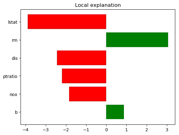
Yay! The prediction locally is identical to the OLS one. But everything else looks, uh, different. What are we looking at here?
- The breakdown of the effects of the features in the locally estimated model (i.e. the weights).
- The intercept, estimate using the local model, and the value predicted by the original OLS
- The prediction of the local model and the base (in this case global OLS) model.
Ok, so all this looks a little different than what we're used to with the OLS. But the difference here is purely one of standardization done by LIME. A quick conversion allows us to compare the local linear model (LIME) to the global one (our original OLS).
| variable_name | value | ols_coef | normed_coef | denormed_coef |
|---|---|---|---|---|
| b | 394.12 | 0.01 | 0.87 | 0.01 |
| dis | 6.06 | -1.16 | -2.44 | -1.16 |
| lstat | 5.21 | -0.55 | -3.89 | -0.54 |
| nox | 0.46 | -15.84 | -1.83 | -15.83 |
| ptratio | 18.70 | -1.01 | -2.19 | -1.01 |
| rm | 6.43 | 4.35 | 3.06 | 4.35 |
Great! As expected, the local linear model is nearly identical to the global one. Now, the standard way to use LIME is to look at the contribution of each variable to the final estimate. This is where a subtle point about the data centering comes in: LIME describes the contribution of each variable relative to the mean of that variable.
In the case of of non-discretized variables, this is not really a big deal. You have to adjust for the standard deviations, but the effect of a change in a feature of interest does not depend on the current value of the feature. Coefficients are easily converted.
However, when interpreting discretized variables, this becomes important (and preferable). Let's take a look:
Discretized Model
Below are the results of rerunning the previous code setting discretize_continuous=True. This is the default method for LIME. This can help interpretability for a couple of reasons. According to Ribiero:[4]
- The values may be in different ranges. We can always standardize the data, but then the meaning of the coefficients changes
- It's hard to think about double negatives (i.e. negative weight for a negative feature = positive contribution)
Of course, this will all depend on your usecase. The ability to determine local elasticities, for instance, could be particularly valuable. (Using LIME as an alternative way of deriving marginal effects).
I'll use two different methods of discretizing: quartile and decile. These represent the number of discrete bins that will be created (i.e. 4 or 10 bins over the range of data).


OLS prediction: 26.24

Local discretized predictions:
Quartile-based: 24.98
Decile-based: 26.20

Intercepts:
Quartile-based: 21.53
Decile-based: 22.09
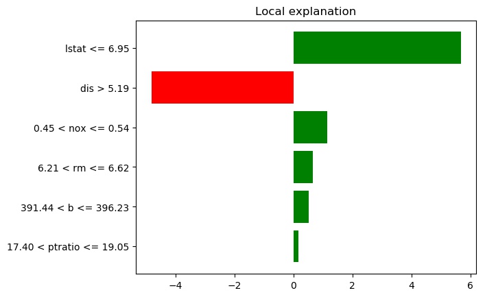
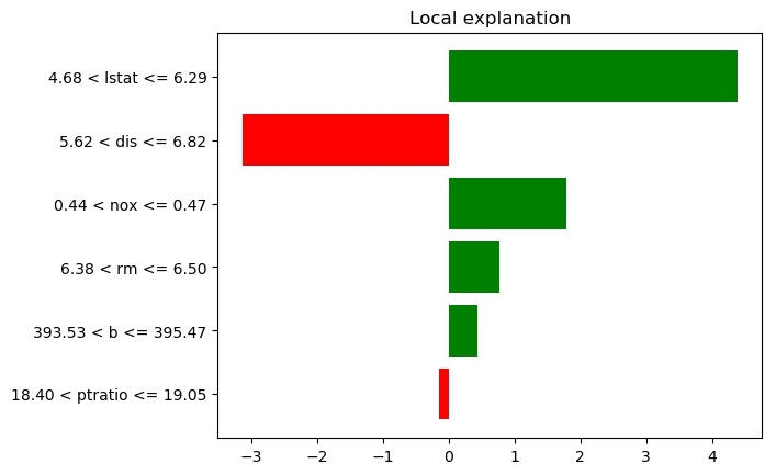
This looks a lot different, understandably: it's trying to estimate a linear model using dummies for whether a variable lies within a certain quartile of the values for that variable in the training set. First off, the local prediction is different this time, and actually further from the "True" prediction of 28.7[5]. Secondly, the effects given are now coefficients on dummies, meaning they can be thought of as the contribution to the prediction.
See the below table for the comparative contributions[6]. The first 2 columns are $$\beta_i * x_i$$, the latter are simply $$\beta_i$$, as explained above.
| variable_name | ols | normed_ols | disc_quartile | disc_decile |
|---|---|---|---|---|
| b | 3.77 | 0.36 | 0.51 | 0.44 |
| dis | -7.02 | -2.63 | -4.82 | -3.13 |
| lstat | -2.84 | 4.06 | 5.67 | 4.39 |
| nox | -7.25 | 1.53 | 1.14 | 1.78 |
| ptratio | -18.91 | -0.25 | 0.18 | -0.15 |
| rm | 27.97 | 0.63 | 0.65 | 0.77 |
| intercept | 30.51 | 22.53 | 21.57 | 22.09 |
As alluded to, the ols contributions are vastly different in magnitude and direction from the other 3 columns. This is because they are based on deviations from the origin, rather than the mean of the data. Although this could be thought of as "objective", it doesn't give a good job of explaining the observation in the context of the model or the data.
For instance, imagine you are running a regression of ice cream sales on ambient temperature, measured in Kelvin. Using the above contribution method, you would have a positive contributions to sales even in the dead of Winter. But it's more helpful to think about it as deviation from the mean temp, with the weather contributing in the summer and hurting sales in the winter.
There are also differences due to standardizing by the standard deviation, but only in interpretation of the actual coefficient. e.g. the coefficient on rm is the effect of one s.d. increase in # of rooms, rather than an increase of 1 room.
Moving to the final 3 columns, they're all pretty similar. The contributions calculated using the discrete decile are, in this case, closer to the normed_ols contributions. This makes sense: using n-tiles, as you increase n to infinity, it will further and further approximate a linear model (given you increase sample size to avoid over-specification issues). But the signs and magnitudes are all quite similar, which is pretty cool!
Conclusion
This has been a fun little foray into how to think about what LIME is producing. but we haven't really seen it in action. Part 2 will focus on applications with different types of models and different mediums (e.g. images).

References
Technically you can have LIME perturb the intercept too. However, LIME will estimate its own intercept (it's creating a local linear model after all), so the estimated effect from LIME from the intercept will be 0. ↩︎
Issue threads: the most unflattering place to reference someone ↩︎
This is completely unsurprising. LIME has no knowledge of the true values -- it is simply trying to model the model. If the local estimate was closer than the original OLS estimate for observation 5, it would be pure happenstance. ↩︎
The first 2 columns I derive from the local estimate -- the denormed and then the normed. Though they are technically different than the true ols estimates, they should be nearly identical as exampled in the previous section. ↩︎